It’s astounding to think back and consider how much technological progress has occurred in just the past 15 years. Most folks today carry a smartphone in their pocket everywhere they go, and a great many of those smartphones have powerful cameras built in capable of recording multiple hours in high definition. Pair this ability with low-cost video editing software—some of which comes at no cost at all—and far more people today have the tools to practice shooting, editing, compositing, and rendering professional-looking videos on a modest budget.
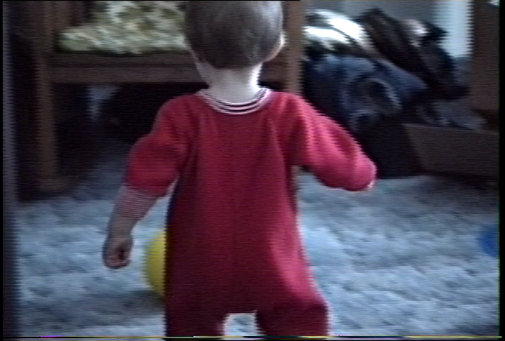
My personal experience with photography began around age 7 shooting on 110 film using a small “spy” camera I got as a gift. My dad’s Sony CCD-V5 was bulky, heavy, and probably expensive when he bought it around 1987, so he was reluctant to let me or my sister operate it under his supervision, let alone borrow it to make our own films by ourselves. As a consequence, my sister and I kept ourselves entertained by making audio recordings on much cheaper audio cassette hardware and tapes—we produced an episodic “radio show” starring our stuffed animals long before the podcast was invented. Though my sister and I took good care of our audio equipment, Dad stuck to his guns when it came to who got to use the camcorder, but he would sometimes indulge us when we had a full production planned, scripted, and rehearsed. Video8 tapes were expensive, too, and for the most part Dad reserved their use for important events like concerts, school graduations, birthdays, and family holidays.

I went off to college and spent a lot of time lurking the originaltrilogy.com forums. It was here that not only did I learn a lot about the making and technical background of the Star Wars films (a topic I could blog about ad nauseum), but I also picked up a lot about video editing, codecs, post-production techniques, and preservation. OT.com was and still is home to a community of video hobbyists and professionals, most of whom share a common love for the unreleased “original unaltered” versions of the Star Wars trilogy. As such, many tips were/are shared as to how to produce the best “fan preservations” of Star Wars and other classic films given the materials available, sacrificing the least amount of quality.
I bought my dad a Sony HDR-CX100 camcorder some years ago to supplement his by that time affinity for digital still cameras—he took it to Vienna and Salzburg soon after and has since transitioned to shooting digital video mostly on his iPhone. But the 8mm tapes chronicling my family’s milestones over the first 25 years of my life continued to sit, undisturbed, in my folks’ cool, dry basement. My dad has recordings on them going as far back as 1988 that I’ve found so far. These recordings are over 30 years old, so the tapes must be at least that age.
8mm video tape does not last forever, but making analog copies of video tape incurs generational loss each time a copy is dubbed. On the other hand, a digital file can be copied as many times as one wants without any quality loss. All I need is the right capture hardware, appropriate capture software, enough digital storage, and a way to play back the source tapes, and I can preserve one lossless digital capture of each tape indefinitely. The last 8mm camcorder my dad bought—a Sony CCD-TR917—still has clean, working heads and can route playback of our existing library of tapes through its S-video and stereo RCA outputs. This provides me with the best possible quality given how they were originally shot.
Generally with modern analog-to-digital preservation, you want to losslessly capture the raw source at a reasonably high sample rate with as little processing done to the source material as possible, from the moment it hits the playback heads to the instant it’s written to disk. Any cleanup can be done in post-production software; in fact, as digital restoration technology improves, it is ideal to have a raw, lossless original available to revisit with improved techniques. For this project, I am using my dad’s aforementioned Sony CCD-TR917 camcorder attached directly to the S-video and stereo audio inputs of a Blackmagic Intensity Pro PCIe card. The capturing PC is running Debian Linux and is plugged into the same circuit as the camcorder to avoid possible ground loop noise.
Since my Debian box is headless, I’m not interested in bringing up a full X installation just to grab some videos. Therefore I use the open source, command-line based bmdtools suite—specifically bmdcapture—to do the raw captures from my Intensity Pro card. I do have to pull down the DeckLink SDK in order to build bmdcapture, which does have some minor X-related dependencies, but I have to pull down the DeckLink software anyway for Linux drivers. I invoke the following from a shell before starting playback on the camcorder:
$ ./bmdcapture -C 0 -m 0 -M 4 -A 1 -V 6 -d 0 -n 230000 -f <output>.nut
The options passed to bmdcapture configure the capture as follows:
-C 0: Use the one Intensity Pro card I have installed (ID 0)-m 0: Capture using mode 0; that is, 525i59.94 NTSC, or 720×486 pixels at 29.97 FPS-M 4: Set a queue size of up to 4GB. Without this, bmdcapture can run out of memory before the entire tape is captured to disk.-A 1: Use the “Analog (RCA or XLR)” audio input. In my case, stereo RCA.-V 6: Use the “S-Video” video input. The S-video input on the Intensity Pro is provided as an RCA pair for chroma (“B-Y In”) and luma/sync (“Y In”); an adapter cable is necessary to convert to the standard miniDIN-4 connector.-d 0: Fill in dropped frames with a black frame. The Sony CCD-TR917 has a built-in TBC (which I leave enabled since I don’t own a separate TBC), but owing to the age of the tapes, there is an occasional frame drop.-n 230000: Capture 230000 frames. At 29.97 FPS, that’s almost 7675 seconds, which is a little over two hours. Should be enough even for full tapes.-f <output>.nut: Write to<output>.nutin the NUT container format by default, substituting the tape’s label for<output>. The README.md provided with bmdtools suggests sticking with the default, and since FFmpeg has no trouble converting from NUT and I’ve had no trouble capturing to that format, I leave the output file format alone.
Once I have my lossless capture, I compress the .nut file using bzip2, getting the file size down to up to a quarter of the original size depending on how much of the tape is filled. I then create parity data on the .bz2 archive using the par2 utility, and put my compressed capture and parity files somewhere safe for long-term archival storage. 🙂
My Windows-based Intel NUC is where I do most of my video post-production work. It lacks a PCIe slot, so I can’t capture there, but that’s fine because at this point my workflow is purely digital and I only have to worry about moving files around. My tools of choice here are AviSynth 2.6 and VirtualDub 1.10.4, but since AviSynth/VirtualDub are designed to work with AVI containers, I first convert my capture from the NUT container to the AVI container using FFmpeg:
$ ffmpeg.exe -i <output>.nut -vcodec copy -acodec copy <output>.avi
The options passed to FFmpeg are order-dependent and direct it to do the following:
-i <output>.nut: Use<output>.nutas the input file. FFmpeg is smart and will auto-detect its file format when opened.-vcodec copy: Copy the video stream from the input file’s container to the output file’s container; do not re-encode.-acodec copy: Likewise for the audio stream, copy from the input file’s container to the output file; do not re-encode.<output>.avi: Write to<output>.avi, again substituting my tape’s label for<output>in both the input and output filenames.
A note about video containers vs. video formats
Pop quiz! Given a file with the .mov extension, do you know for sure whether it will play in your media player?
Files ending with .mov, .avi, .mkv, and even the .nut format mentioned above are “container” files. When you save a digital video as a QuickTime .mov file, the .mov file is just a wrapper around your media, which must be encoded using one or more “codecs.” Codecs are small programs that can encode and/or decode audio or video. These codecs must be specified at the same time as when you save your movie. QuickTime files can wrap among a great many codecs: Motion JPEG, MPEG, H.264, and Cinepak just to name a few. They’re a bit like Zip files, except that instead of files inside you have audio and/or video tracks, and there’s no compression other than what’s already done by the tracks’ codecs. Though Apple provides support in QuickTime for a number of modern codecs, older formats have been dropped over time and so any particular .mov file may or may not play… even using Apple’s own QuickTime software! Asking for a “QuickTime movie” is terribly vague—a QuickTime .mov file may not play properly on a given piece of hardware if support for a containing codec is missing.
AVI, MKV, and MP4 are containers, too—MP4 is in fact based on Apple’s own QuickTime format. But these are still just containers, and a movie file is nothing without some media inside that can be decoded. Put another way, when I buy a book I’m often offered the option of PDF, hardcover, or paperback form. But if the words contained therein are in Klingon, I still won’t be able to read it. When asked to provide a movie in QuickTime or AVI “format,” get the specifics—what codecs should be inside?
Now that I have an AVI source file, I can open it in VirtualDub. Owing to its namesake, VirtualDub’s interface is reminiscent of a dual cassette deck ready to “dub” from one container to another. It isn’t as user-friendly as, say, Premiere or Resolve when it comes to editing and compositing, but what it lacks in usability it gains in flexibility. In particular, VirtualDub is designed to run a designated range of source video through one or more “filters,” encoding to one of several output codecs available at the user’s discretion via Video for Windows and/or DirectShow. If no filters are applied, VirtualDub can trim a video (and its audio) without re-encoding—great for preparing source footage clips for later editing or other processing.

Though the Sony CCD-TR917 has a built-in video noise reduction feature, I explicitly turn it off before capturing, because one of the filters I have for VirtualDub is “Neat Video” by ABSoft. It’s the temporal version of their “Neat Image” Photoshop filter for still images, which I used most recently to prepare a number of stills for Richard Moss’s The Secret History of Mac Gaming. It’s a very intelligent program that has a lot of knobs and dials to really tune in the noise profile you want to filter out, so I was equally delighted to find that ABSoft’s magic works on videos too. Luckily they offer a plugin built to work with VirtualDub, so I didn’t hesitate to buy it as a sure improvement over the mid-90s noise reduction technology built in to the camcorder.
Most of the aforementioned features can be done in high-end NLE applications such as Resolve—indeed I have used Resolve to edit several video projects of my own. What makes VirtualDub the “killer app” for me is its use of Windows’s built-in video playback library, and therefore its ability to work with AviSynth scripts. AviSynth is a library that can be installed on Windows PCs that grants the ability to interpret AviSynth “script” files (with the .avs extension) as AVI files anywhere Windows is prompted to play one using its built-in facilities. The basic AviSynth scripting language is procedural, without loops or conditionals, but it does retain the ability to work with multiple variables at runtime and organize frequently-called sequences into subroutines. Its most common use is to form a filter chain starting with one or more source clips, ending with a final output clip. When “played back,” the filter chain is evaluated for each frame, but this is transparent to Windows, which instead just sees a complete movie as though it’s already rendered to an AVI container.
Combined with VirtualDub, AviSynth allows me to write tiny scripts to do trims and conversions with frame-accurate precision, then render these edits to a final output video. Though AviSynth should be able to invoke VirtualDub plugins from its scripting language, I couldn’t figure out how to get it to work with Neat Video, so I did the next best thing: I created a pair of AviSynth scripts; one to feed to Neat Video, and one to process the output from Neat Video. The first script looks like this:
AviSource("1988 Christmas.avi")
# Invoke Neat Video
ConvertToRGB(matrix="Rec601", interlaced=true)
Absent of an explicit input argument, each AviSynth instruction receives the output of the previous instruction as its input. The Neat Video plugin for VirtualDub expects its input to be encoded as 8-bit RGB. VirtualDub will automatically convert the source video to what Neat Video expects if not already in the proper format. Since I’m not sure exactly how VirtualDub does its automatic conversion, I want to retain control over the process so I do the conversion myself from YUV to RGB using the Rec.601 matrix. I know that my source video is from an interlaced analog NTSC source; VirtualDub doesn’t know that unless I explicitly say so.
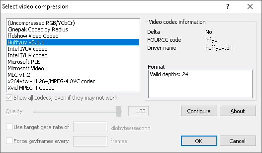
I render this intermediate video to an AVI container using the Huffyuv codec. Huffyuv is a lossless codec, meaning it can compress the video without any generational loss. Despite its name, Huffyuv is perfectly capable of keeping my video encoded as RGB. I can’t do further AviSynth processing on the result from Neat Video until I load it into my second AviSynth script, so I’m happy that its output can be unchanged from one script to the next.
Color encodings and chroma subsampling
Colors reproduced by mixing photons can be broken down into three “primary colors.” We all learned about these in grade school: red, green, and blue. Red and blue make purple, blue and green make turquoise, all three make white, and so on.
On TV screens, things are a bit more complicated. Way back when, probably before you were born, TV signals in the United States only came in black and white, and TVs only had one electron gun responsible for generating the entire picture. The picture signal mostly comprised of a varying voltage level per 525 lines indicating how bright or dark the picture should be at that point in that particular line. The history of the NTSC standard used to transmit analog television in the United States is well-documented elsewhere on the Internet, but the important fact here is that in 1953, color information was added to the TV signal broadcast to televisions conforming to the NTSC standard.
One of the challenges in adding color to what was heretofore a strictly monochrome-only signal was that millions of black and white TVs were already in active use in the United States. A TV set was extremely expensive even by the early 1950s, so rendering all the active sets obsolete by introducing a new color standard would have proven quite unpopular. The solution—similar to how FM stereo radio was later standardized in 1961—was to add color as a completely optional, but still integral, signal of monochrome TV. The original black and white signal—now known as “luma”—would continue to be used to determine the brightness or “luminance” of the picture at any particular point on the screen, while the new color stream—known as “chroma”—would only transmit the color or “chrominance” information for that point. Existing black and white TVs would only know about the original “luma” signal, and so would continue to interpret it as a monochrome picture, whereas new color TVs would be aware of and overlay the new “chroma” stream on top of the original “luma” stream to produce a rich, vibrant, color picture. All of this information still had to fit into a relatively limited bandwidth signal, designed in the early 1940s to be transmitted through the air with graceful degradation in poor conditions.
The developers of early color computer monitors, by contrast, needed not worry about maintaining backward compatibility with black and white American television nor did they need to concern themselves with adopting a signal format that was almost 50 years old by that point. It should be of little surprise then, naturally, that computer monitors generate color closer to how we learned in grade school. Computer monitors in particular translate a signal describing separate intensities of red, green, and blue to a screen made up of triads of red, green, and blue dots of light. This signal describing what’s known as “RGB” color (for Red, Green, and Blue) comes both from that aforementioned color theory of mixing primaries, but also historically from those individual color signals more or less directly driving the respective voltages of three electron guns inside a color CRT. Despite both color TVs and computer monitors having three electron guns for mixing red, green, and blue primary colors, the way that color information is encoded before entering the TV is a main differentiator.
Whereas RGB is the encoding scheme by which discrete Red, Green, and Blue values are represented, color TV uses something more akin to what’s known as “YUV.” YUV doesn’t really stand for anything—the “Y” component represents Luma, and the “UV” represents a coordinate into a 2D color plane, where (1, 1) is magenta, (-1, -1) is green, and (0, 0) is gray (the “default” value for when only the “Y” component is present, such as on black and white TVs). In NTSC, quadrature amplitude modulation is used to convey both of the UV components on top of the Y component’s frequency—I don’t know exactly what quadrature amplitude modulation is either, but suffice it to say it’s a fancy way of conveying two streams of information over one signal. 🙂
An interesting quirk of how the human visual system works is that we have evolved to be much more sensitive to changes in brightness than in color. Some very smart people have sciencey explanations as to why this is, but ultimately we can thank our early ancestors for this trait—being able to detect the subtlest of movements even in low light made us expert hunters. Indeed, when the lights are mostly off, most of us can still do a pretty good job of navigating our surroundings (read: hunting for the fridge) despite there being limited dynamic range in the brightness of what we can see.
Note that having a higher sensitivity to brightness vs. color does not mean humans are better at seeing in black and white. It merely means that we notice the difference between something bright and something dark better than we can tell if something is one shade of red vs. a different shade of red. In addition, humans are more sensitive to orange/blue than we are to purple/green. These facts actually came in very handy when trying to figure out how to fit a good-enough-looking color TV signal into the bandwidth already reserved (and used) for American television. Because we are not as sensitive to color, the designers of NTSC color TV could get away with transmitting less color information than what’s in the luma signal. By reducing the amount of bandwidth for the purple/green range, color in NTSC can still be satisfactorily reproduced, though the designers of NTSC adopted a variant of YUV to accomplish this called “YIQ.” In YIQ, the Y component is still Luma, but the “IQ” represents a new coordinate into the same 2D color plane as YUV, just rotated slightly so that the purple/green spectrum falls on the axis with a smaller range. Nowadays with the higher bandwidth digital TV provides, we no longer need to encode using YIQ, but due again to the way our vision system responds to color and the technical benefits it provides, TV/video is still encoded using YUV, albeit will a fuller chroma representation.
What does all of this have to do with digitizing old 8mm tapes?
Each pixel on a modern computer screen is represented by at least three discrete values for Red, Green, and Blue. Though NTSC defines 525 lines per frame (~480 visible), being an analog standard means there really isn’t such a thing as “pixels” horizontally. However, most capture cards are configured to sample 720 points along each line of NTSC video, forming what we would call 720 “pixels” per line. But two important details must be noted:
- Though 720 samples are enough to effectively capture the entire line, only 704 of them are typically visible and furthermore, NTSC TV is designed for a 4:3 aspect ratio. That is, if the picture is 480 square dots vertically, then it must be
(480 * 4) / 3 == 640square dots horizontally, or the picture will appear squished and everything will look “fat.” A captured NTSC frame at 720×480 will need horizontal scaling plus cropping to 640×480 to be displayed with the correct aspect ratio on a computer screen with square dots. - 720 samples are enough to capture each line of the luma component. The chroma component is a whole other story.
Remember how the luma and chroma components are encoded separately, but that some of the chroma information can be discarded to save space and we’re not likely to notice? Turns out, computers can use that technique too to reduce bandwidth usage and save disk space. RGB is just how your computer talks to its display, but there’s no rule that says computer video files need to be encoded as RGB. We can encode them as YUV, too, and this is where the term chroma subsampling comes in.
While we always want to sample all 704 visible “pixels” of luma information, we can often get away with capturing 50% or even as little as 25% of the chroma information for a given line of picture. The ratio of sampled chroma data to luma data is called the “chroma subsampling” ratio and is indicated by the notation Y:a:b, where:
Y: the number of luma samples per line in the conceptual two-line block used byaandbto reference. This is almost always 4.a: the number of chroma samples mapped over thoseYdots in the first line. This is at mostY.b: the number of times thoseachroma samples change in the second line. This is at mosta.


A chroma subsampling ratio of 4:4:4 means that every luma sample has its own distinct chroma sample; this ratio captures the most data and therefore provides the highest resolution. The value of a is directly proportional to the horizontal chroma resolution, and the value of b is directly proportional to the vertical chroma resolution. NTSC is somewhere between 4:1:1 and 4:2:1 (consumer tape formats even less), whereas the PAL standard in Europe is closer to 4:2:0 (half the vertical chrominance resolution as NTSC). As the values of a and b shrink, the overall chroma resolution decreases, and depending on your source picture it may be more or less noticeable.
As the chroma resolution on this photo of Annie is diminished, artifacts become apparent which should remind you of heavily-compressed JPEG images. This is no coincidence—the popular JPEG image codec and all variants of the popular MPEG video codec use YUV encoding and discard chroma data as a form of compression. This is one reason why encoding as YUV is popular with real-world images and video—an RGB representation can be reconstructed by decoding the often-smaller YUV information, much like a color CRT has to do to get a YUV-encoded picture on its screen through its RGB electron guns. A ratio of 4:2:0 is popular with the common H.26x video codecs (though H.26x can go up to a full 4:4:4), and several professional codecs indicate their maximum chroma subsampling ratios directly in the name of the codec. DNxHR 444 and ProRes 422 come to mind. What these numbers represent is how much chroma information can be preserved from the original, uncompressed image, but looking at it another way, they represent how much chroma information is discarded during compression.
Breaking it down further, we can see how various chroma subsampling ratios affect the chroma information saved (or not) in this close-up of Annie’s toys. Notice the boundary between the pink and green halves of her ball, and the rightmost edge of her red and white rolling cage.
With my analog NTSC 8mm tapes having chroma resolution of at most 50% of the luma resolution, I need to capture them with at least a 4:2:0 chroma subsampling ratio. That 50% could be in the horizontal direction, the vertical direction, or both, but fortunately bmdcapture grabs YUV video at a 4:2:2 chroma subsampling ratio from my Blackmagic Intensity Pro card by default, which is enough to sample all the chroma information in my NTSC source. This is fine for my 8mm tapes, but if I want to capture a richer video signal in the future (like, say, a digital source over HDMI), I would probably want to investigate capturing at a full 4:4:4 ratio.
I tell Neat Video to clean up my interlaced video with a temporal radius of 5 (the maximum) and a noise profile I generated in advance for the Sony CCD-TR917 I’m using. With these parameters, it takes about eight hours to clean up two hours of raw footage on my PC, so I usually start it in the morning and have it running in the background while I work during the day. Once it’s finished, I’m ready to feed its intermediate result to my second and final AviSynth script to get my final output:
AviSource("1988 Christmas NV.avi")
ChangeFPS("ntsc_video")
ConvertBackToYUY2(matrix="Rec601")
QTGMC(Preset="Placebo", MatchPreset="Placebo", MatchPreset2="Placebo", NoiseProcess=0, SourceMatch=3, Lossless=2)
# Trim the fat
Trim(329, end=222768)
# Crop to 704x480
Crop(4, 0, -12, -6)
For some reason, Neat Video produces two identical frames for every input frame I provide in the first script, so the first step in the second script tells AviSynth to disregard those duplicate frames and assume we’re dealing with a 59.94 Hz interlaced NTSC video. I then convert Neat Video’s intermediate RGB result back to its original YUV encoding, once again using the Rec.601 matrix corresponding to my video’s NTSC format.
ConvertBackToYUY2
YUY2 is a digital representation of YUV-encoded video, using 16 bits per pixel. When capturing with a chroma subsampling ratio of 4:2:2, each chroma sample is shared with two luma samples. YUY2 encodes this by reserving 8 bits for each of four luma samples (“Y”), then 16 bits for each of the two chroma samples (8 bits for each of the two components of “UV”). When you add it all up, 8 bits x 4 luma samples + 16 bits x 2 chroma samples == 64 bits. Divide that by the four luma samples and you get 16 bits per pixel.
Before calling ConvertToRGB in the first script, our original raw capture was encoded as uncompressed YUV 4:2:2. ConvertToRGB does a bit of math to map the YUV values into RGB space given the conversion matrix specified. If you are converting back to YUY2 from an RGB clip created by AviSynth, using ConvertBackToYUY2 can be more effective because it is allowed to make assumptions about the algorithm initially used to convert to RGB, given that both functions belong to AviSynth. In particular, ConvertBackToYUY2 does a point resampling of the chroma information instead of averaging chroma values as ConvertToYUY2 would, resulting in a chroma value closer to that in the original pre-RGB source clip.
After cleaning up the noise with Neat Video, to prepare these videos for playback on a progressive scan display such as a PC, mobile device, or modern TV, I still need to apply a deinterlacing filter. Each NTSC frame is split into two “fields”—the first field alternates every other line, and the second field has the other half. NTSC only has enough bandwidth to transmit 29.97 frames per second, so interlacing is a trick used to send half-sized “fields” at twice the rate. CRT TVs have a slower response time than modern digital TVs, so the net effect of interlacing on CRTs is that one field “blurs” into the next, producing the illusion of a higher rate of motion. Nowadays when TVs receive an analog NTSC signal they’re smart enough to recognize that it’s interlaced and apply a simple deinterlacing filter. But such filters are designed to work in real time, and without one, an interlaced source will appear to stutter when compared to its deinterlaced 60 Hz counterpart. A free third-party AviSynth script called QTGMC can do a much higher-quality job of deinterlacing ahead of time, with the caveat that I need to apply this script in advance and offline, that is, not in real time.


Here’s something to know about me. When it comes to filtering and rendering media offline, it doesn’t matter to me all that much how long it takes. The only deadline I have with this stuff is the eventual deterioration of the source media (and my own mortality, I suppose). For the moment, I have time and computing cycles to burn. As with the eight-hour Neat Video process, I have no qualms about backgrounding a rendering queue and letting it run overnight or even well into the next day. So when QTGMC and other tools advertise “Placebo” presets, I use them. I sleep better at night knowing there’s nothing more I could do to get a better result out of my tools, however miniscule. 🙂
I finally trim the start and end of my raw capture, leaving only the actual content behind. The last step crops some “garbage” lines from the bottom (VBI data I don’t need to save, but my Blackmagic card captures anyway), along with some black bars on the left and right sides of the image. Not surprisingly, the final dimensions of the video come out to 704×480: the visible part of a digitally-sampled NTSC frame. I render the whole thing out as a lossless Huffyuv-encoded AVI once again, saving the final lossy encoding step for FFmpeg.
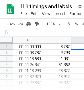
At this point, I have a couple of directions I can take. I can prepare my final video for export to DVD, or I can split my video into one or more video files suitable for uploading to my Plex server. I can do both if I want. In either case, I need to prepare chapter markers so FFmpeg knows how to split the final, monolithic video into its constituent clips. I use Google Sheets for this; I have one sheet with columns for “Start time,” “Duration,” “End time,” and “Label.” I put the “Start time” column in the HH:mm:ss.SSS format that FFmpeg expects for its timecodes, and I express the “Duration” column in seconds with decimals. When I’ve marked all the chapters (relying on VirtualDub’s interface for precise frame numbers and timing), I pull the “Start time” and “Duration” columns into a new sheet and export to a CSV file.
I wrote a handful of Windows batch scripts that take this CSV file, a path to FFmpeg, and a path to my final video, and split my final render into a collection of H.264-encoded MP4 files, or a series of MPEG files encoded for NTSC DVD. In the DVD version, I also generate an XML file suitable for import into dvdauthor. I found that neither my iPhone nor my Android devices like H.264 files encoded with a chroma subsampling ratio higher than 4:2:0, so I wrote a script specifically to encode videos destined for mobile devices. These scripts are longer than make sense to post inline here, so here are links to each one if you’re curious and would like to use them:
Capturing and digitizing my family’s movie memories will help preserve these moments so they can be enjoyed in the years to come without wearing out the original tapes. The biggest cost to this digitization process is time, both in capturing from tape (which is always done in real time) and the offline clean up and encoding to digital files. I still have more than a couple dozen tapes to sort through, so this blog post doesn’t signify the end of this project, but now that I have a reliable process that results in what I consider a marginal improvement over the source material, I like to think I can get through the remaining tapes on a sort of “autopilot.”
I hope this post will inspire someone else to preserve their own memories.
Bonus postscript: field order
As I mentioned above, an interlaced NTSC frame is split into two “fields,” with each field alternating between even and odd lines of the full frame. But which field is sent first? The even field, or the odd field?
The answer, as one might expect, is “it depends.” For my purposes here, the fields in a 480i NTSC signal are always sent bottom field first. But a 1080i ATSC signal—as is used with modern digital TV broadcasts—sends interlaced frames top field first. If you crop the source video before deinterlacing, you have to be careful to crop in vertical increments of two lines, or you run the risk of throwing off the deinterlacer’s expected field order. For example, if line 12 is the first visible line of the first field of my picture, it’s reasonable to expect it to be the bottom field of the frame. After cropping 13 lines from the top of the frame, though, the deinterlacer will assume that line 13 is the bottom field, when it really is the top field. The deinterlacer will then assume that the previous frame is the current frame and will get confused, resulting in motion that appears jerky.
If you must crop an interlaced source by an odd number of lines, AviSynth fortunately has functions to assume a specific field order. AssumeTFF, as its name implies, tells AviSynth that an interlaced clip is Top Field First. Its complement, AssumeBFF, tells AviSynth that a clip is Bottom Field First, though for raw analog NTSC captures this function is largely unnecessary.
Not sure which order is correct for a particular clip? Try deinterlacing in one order, and if the motion looks jerky, try the other. If the motion is smooth, the order is correct.


Alternatively, avoid capturing from interlaced sources altogether. 😛
Good explanation! Thank you
Wow! That was VERY interesting and well written. I’ve learned a lot and will bookmark and reread. For any Apple users looking for a lossless editor like VirtualDub, try this… https://mifi.no/losslesscut/